I have been writing a lot of “did you know” articles as part of our Microsoft Teams reintroduction, and I have an Excel file that lists topics for which we want articles. To avoid posting the same article twice (or worse, writing the same article twice!), I mark off when the article is written and posted. With a long list, though, it is difficult to identify which articles still need to be posted (yeah, I know I’m not apt to have posted an article that hasn’t been written so I could have just used a filter on the ‘Posted’ column … but there are plenty of cases where a simple filter does not suffice). Sometime you can build an advanced filter that isolates the specific data you need, but there’s an easier way — the Excel IF function.

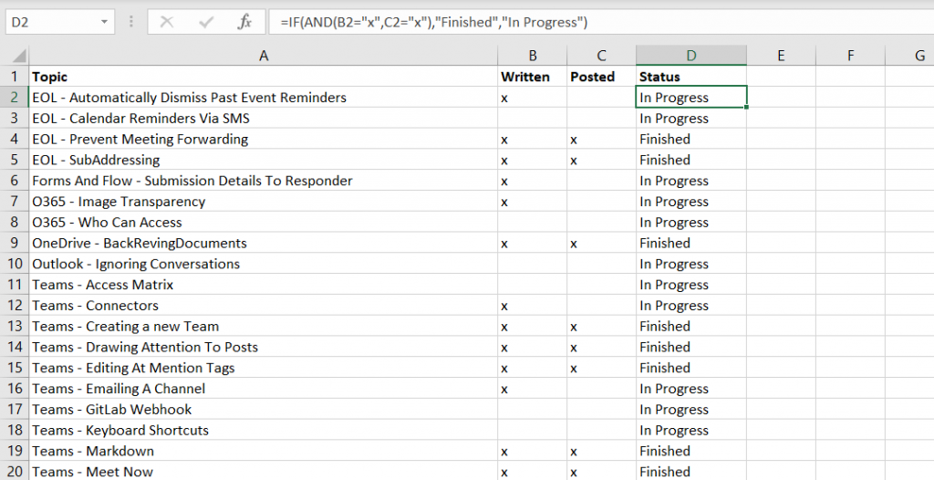
In my spreadsheet, I added a column, named “Status”. The “IF” function displays different text when the test evaluates to TRUE and FALSE: if(B2=”x”,”Written”,”Not written”) displays “Written” in all of the rows where column B has an x, and “Not written” in the remaining columns.

In conjunction with IF, I can use the Boolean AND function to display “Finished” in any row where both columns B and C contain an X:      =IF(AND(B2=”x”,C2=”x”),”Finished”,”In Progress”)

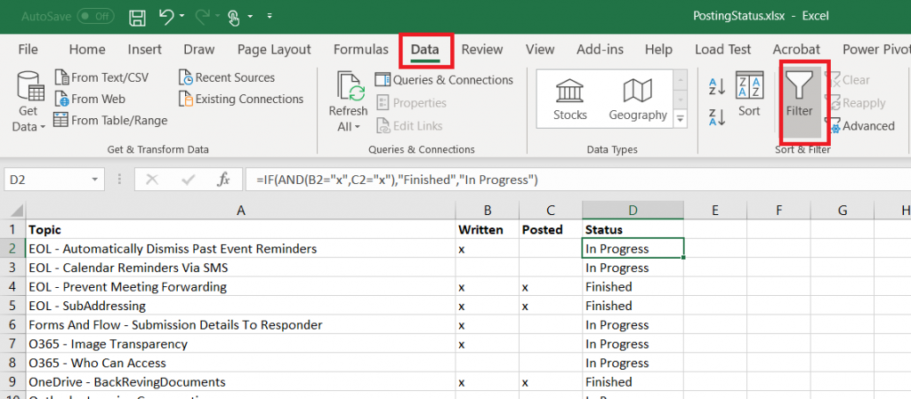
The content of the Status cells can be used as a filter. On the “Data” tab, select “Filter”.

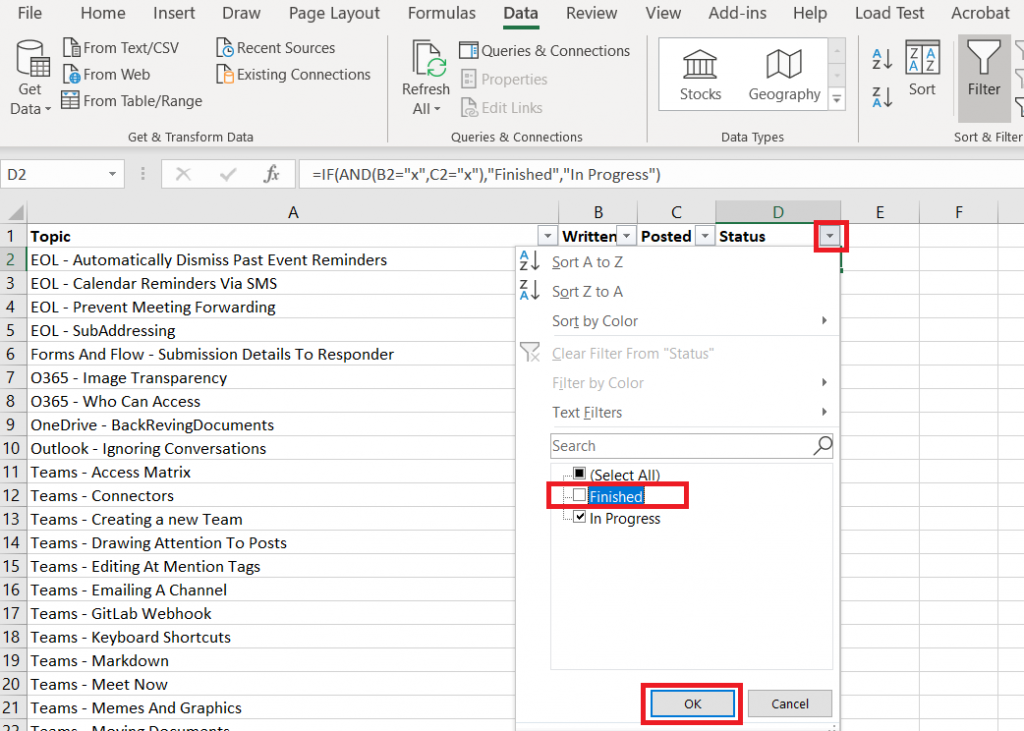
Click the drop-down menu on the “Status” column, deselect whatever values you do not wish to display, then click “OK”.

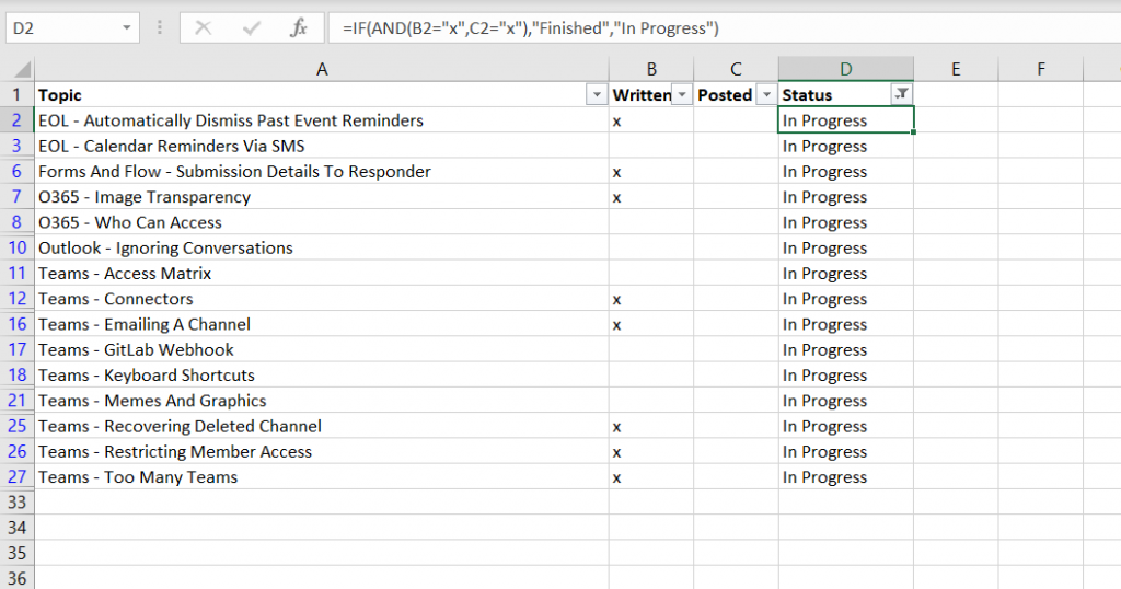
Voila! Now I see only the articles where the status is not “Finished”.